Determining the Maximum Load Capacity and Throttle Point of an HTTP Server Using Grafana K6 – Part 1: Setup and Test Planning

We will see how to set up K6, InfluxDB, and Grafana-server to test an HTTP server’s maximum load capacity before it starts throttling. We’ll cover the installation, motivation and all the set-up.

Introduction

Load testing is essential for ensuring the reliability and scalability of an HTTP API server. Using Grafana K6, we can determine the maximum number of requests per second (RPS) our server can handle before performance degradation occurs. Breakpoint testing helps identify system limits. Reasons for conducting such tests include:

1. Identifying and addressing system bottlenecks to increase performance thresholds.

2. Planning remediation strategies for when the system approaches its limits.

This blog provides a step-by-step guide on setting up and conducting a load test to identify that threshold.

The techniques described here broadly apply to HTTP APIs, including machine learning model inference services or this VIN decoder API, but not to browser-based testing using k6/experimental/browser.

If you are unfamiliar with K6 and its terminology, refer to these resources, K6-docs-url-1, K6-docs-url-2, K6-docs-url-3, K6-youtube-video-1 and K6 forums is a great place to learn and ask questions, a post on VU and iterations. You may also checkout their blog.

Environment Setup before running the tests

We have a server that we want to load test, and we write tests using K6. How do we determine the throttle point of the server? A dashboard displaying key performance metrics, such as request duration over time, would be invaluable.

K6 supports exporting test results as an web dashboard and at the end of the test to a HTML report, offering comprehensive insights. However, these reports are not customizable, limiting our ability to analyze data in ways suited to enterprise needs. like the summary that can be seen at the end of the test is customisable for the intervals, if k6 let’s us customise and add better graphs and heatmaps, I would personally move away from InfluxDB.

For example, we may want:

• A greater percentile-based distribution of request durations over time.

• A breakdown of request durations at specific time intervals, such as how many of the 20K requests sent in a second, were returned in 10ms, how many in 20ms and so on. That bucketised breakdown would help a lot.

• dashboards with graphs which we can customise to get the information needed

• with grafana-dashboards, we will be able to see the the percentiles of http-req-duration, per second that is, instead of an average on k6’s html export per second, you see it in more granular view, like mean (matching with k6’s html), 90, 95, 99 and all that you add, letting you see a view with the effect of the outliers eliminated.

• or even instead of having to just fix to some fixed threshold numbers for the percentiles, we can see heatmaps of the requests per time interval, which is going to help us in a great way with our conclusions.

• Also, let’s you look at a graph with multiple axis, which could be overlap of VUs, RPS and http-req-duration, per second and that can also tell you (along with stderr logs of the load-test) if your request-rate was limited by the hardware on which the test was ran.

• all that is fine, but the only disadvantage (apart from cost and maintenance) that I see with grafana-server (and InfluxDB) is the sql queries that are run and the aggregations used for the visualisations on dashboards can get slow, especially if you have more than a couple of million requests in total for the time-interval chosen. Another biggest problem is, I don’t know from which side, for all the long tests that I have done, metrics were not sent to InfluxDB, sometimes 7 to 11 minutes from the middle of the test went missing strangely and this happened even with K6’s html export.

These insights are not available, at least in the way I described above, in K6’s default exports. The solution is Grafana dashboards, which are highly customizable and can show dashboards by taking data from various sources. In this setup, we use InfluxDB, a time-series database supporting SQL-like queries, where K6 pushes real-time metrics and setup would look something like below,

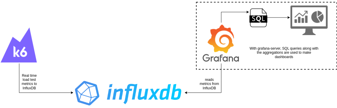
Setup Overview

In a production environment, HTTP API servers typically reside in a private network within an enterprise or a Virtual Private Cloud (VPC). Similarly, InfluxDB and Grafana are hosted on dedicated machines, with K6 tests executed from a separate system—such as a UAT setup, a CI/CD pipeline, or Grafana Cloud or even a developer’s computer.

For this demonstration, all components (the HTTP server, K6, InfluxDB, and Grafana) run on a local Debian 12 machine (actually an c6a.4xlarge AWS EC2 instance which is powerful enough for a few thousand VUs). Consequently:

• No HTTPS is used, which skips TLS overhead completely (real-world scenarios may experience additional delays).

• The HTTP server is accessed via localhost, making metrics like http_req_blocked and http_req_connecting artificially lower than they would be with public IPs or URLs compared to public APIs that involve DNS queries. Also note that K6 caches DNS.

Installing Required Tools

These applications can be installed using tar.gz, .deb, apt etc, on GNU Linux. Windows and Mac users can install equivalent .exe or .dmg files from their respective download pages.

1. Grafana-K6’s OSS - download from here,

2. InfluxDB’s OSS - download from here or here and a configuring guide.

   1. This blog uses InfluxDB v1, as K6 natively supports exporting metrics to it. If you need to use InfluxDB v2, consider the grafana/xk6-output extension.

   2. After installation, start InfluxDB and create a database for storing K6 metrics:

      $ influx -host=localhost -port=8086
      Connected to http://localhost:8086 version v1.11.8
      InfluxDB shell version: v1.11.8
      > create database k6_latency_tests
      > show databases
      name: databases
      name
      ----
      _internal
      k6_latency_tests

   3. If you plan to run tests with thousands of Virtual Users (VUs), ensure that InfluxDB is hosted on a scalable machine and configured with an appropriate push interval to handle high request volumes for the database to be able to take in the raw metrics of hundreds of thousands (or millions) of requests from K6.

3. Grafana-server for dashboards - download from here and setup guide.

   1. After installation, start the server $ sudo systemctl start grafana-server, and you will then be able to access the dashboard at URL http://localhost:3000.

   2. Go to the dashboards section from the left pane to import an existing JSON dashboard or create one from scratch. This blog uses a custom dashboard adapted from community dashboards 2587 and 19179. And it will be provided on my github-repo.

Start the grafana-server by running sudo systemctl start grafana-server or by double-clicking the icon on your desktop, then go to “http://localhost:3000/dashboards” on your browser to access dashboards. If you are accessing this for the first time, you will have to sign-in too, username and passwords are admin and admin, which can be changed. Then add the InfluxDB as data source by following this guide on influxdata’s docs (which should also walk you through on how to use influx to connect to the db and run sql queries) and navigate to section “Grafana and InfluxDB connection setup”. Then after that, import a dashboard by following these steps on grafana’s docs.

Alternative Setup Using Docker

If you prefer using Docker, start with this docker-compose setup, modify the image loadimpact/k6 to grafana/k6 and adjust other configurations as needed. However, for this demonstration, I avoid Docker to conserve compute resources for running the HTTP server, K6, and InfluxDB. Ensure that the compute resources are distributed appropriately among the containers run.

I will include my config files of InfluxDB and Grafana, on my GitHub repository.

Motivation and set up for the Load Test

The outcome or inference expected is, When the server is in production, processing user requests, we want to determine the approximate number of requests at which it throttles—leading to increased latency or even request timeouts, which negatively impact user experience.

To simulate real conditions, the test includes multiple stages:

1. Linear RPS Growth – Requests per second (RPS) increase steadily to observe how latency evolves as RPS rises.

2. Sudden RPS Spikes – Simulating peak loads during certain times of the day, such as mornings.

3. Cool-Down Periods – Representing times of relatively lower traffic, such as nights.

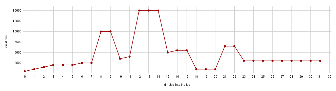
These stages help us determine when the server can respond within <5ms and when latency starts exceeding 1-2 seconds or even timing out. To determine that, precise RPS values are crucial, I will be using the constant-arrival-rate executor, ensuring predictable RPS every second during the test. Using other scenarios results in unpredictable RPS, making it harder to establish a clear correlation between X RPS → M ms of latency and Y RPS → N ms of latency. This becomes evident in the test results visualized through graphs in later sections of the blog. And for this very reason, https://k6.io/blog/how-to-generate-a-constant-request-rate-with-the-new-scenarios-api/ also tells the same thing.

The key parameters for the constant-arrival-rate executor include rate, timeUnit, duration, and preAllocatedVUs. For example, setting rate=100, timeUnit='1s', and duration='1m' results in approximately 100 API requests per second. The preAllocatedVUs parameter ensures that a sufficient number of VUs are available to handle the load without delays due to VU initialization.

If the test environment lacks enough VUs, a warning like WARN[0002] Insufficient VUs, reached <number> active VUs and cannot initialize more executor=constant-arrival-rate scenario=<scenario-name> will appear. Unlike traditional VU-based approaches, where VUs are spawned dynamically and may waste resources, constant-arrival-rate maintains precise control over RPS without unnecessary overhead. ramping-arrival-rate also might seem like a good candidate, but by the definition, it works a bit differently. Going by the same parameters as above (rate is target here, so, target=100`, `timeUnit='1s'`, and `duration='1m'`), RPS will reach100 by the end of the 1 minute, that means, its a gradual increase by the end of set duration, unlike with constant-arrival-rate, rate of RPS will remain consistent through out the set duration of the stage, which I believe is a better way of judging, however you are free to choose ramping-arrival-rate or any other executor/scenario, but aim to have a predictable number of RPS.

About the server being load-tested:

1. The server that I will be testing is a machine-learning inference server hosted on localhost and you are fee to use anything else.

2. Do not do this testing with a server hosted in an elastic cloud environment which is designed to grow with the load (so, do not use https://test.k6.io/), consequently you will find the limit of your cloud account bill, not the load it can handle. So, I would strongly recommend you to turn off elasticity on all the components in the API pipeline, or remember to set hard limits if checking the elasticity is one of your objectives with this test.

3. I won’t be using only input (or payload) for the entire load test, but 4 inputs, since having more, like say a dozen in itself would make the test script long or even any number of inputs won’t be able to replicate the real variance in the millions of requests that the server expects every day, so I will stick to just 4 and choose one randomly for each request. And since, we only have 4 inputs, enabling cache will make the results, especially http_req_duration extremely optimistic, so I will not have any of the caching the server.

4. Also, if you have cache enabled for similar inputs to the API, you are likely to get optimistic results of the latency (http_req_duration). No cache is enabled in the HTTP server, due to which I would get right numbers for http_req_duration, since for a load test. And for similar reasons, I also have connection-reuse turned off from server and also in K6 (by setting the options, noConnectionReuse and noVUConnectionReuse to true).

5. This server relies heavily on CPU/GPU and not a lot on RAM (for storing model and tensors) and minimal I/O (model is read from disk only once before the server starts), given that this is a scripted pytorch or libtorch model being run with cpp-httplib.

In the next part, we will,

1. put together the load-test script

2. run the test by taking care of few things

3. set up and go through the dashboard to interpret the results and make inferences about the load-handling capacity of our HTTP server.