Determining the Maximum Load Capacity and Throttle Point of an HTTP Server Using Grafana K6 – Part 2: Running Tests and Analyzing Results

Execute a K6 load test, collect metrics in InfluxDB, and visualize them in Grafana. And analyze response times, error rates, and throughput to identify when server reaches its limit and throttles.

Brief Recap:

In the previous part, we discussed:

• Introduction, environment setup, and software installation.

• Motivation for designing the tests to support our inferences.

Load testing script

Components of the Load Testing Script:

1. For default function:

   1. Sample input (or body) to send to the server.

2. Variables outside options and the default function, such as URL and headers.

3. For options:

   1. Stages using constant-arrival-rate, executed consecutively.

   2. Summary statistics and thresholds for quick verification before analyzing dashboards.

Let's examine the components from smallest to largest;

Static Components:

const url = 'http://0.0.0.0:8080/predict';
const headers = {'Content-Type': 'application/json'};

Note: I did not include Connection: keep-alive because ML inference APIs typically handle fresh requests from new users. If your application expects sustained loads, feel free to add it.

Inputs

The API expects a dictionary containing a 3×4 matrix.

const payload_01 = { "input_matrix": [[[0.3879, 0.2045, 0.2850, 0.4871], [...], [0.0631, 0.5948, 0.9220, 0.1469]]] };

I'll use four different payloads, randomly selecting one for each request in the default function:

const all_payloads = [payload_01, payload_02, payload_03, payload_04];

Inside the default function:

all_payloads[Math.floor(Math.random() * 4)];

Writing default function

The function is straightforward. it sends a request with a randomly chosen payload from one of our 4 inputs and checks if the response status is 200, which should constitute as one iteration.

export default function () {
    let response = http.post(url, JSON.stringify(all_payloads[Math.floor(Math.random() * 4)]), {headers});

    // ensure that the ouptut status is 200
    check (response, {
        'status is 200': response.status === 200,
        // 'output contains relevant keys': response.json() === 200,
    });
}

If you don't need to check the status code or process the response, you can set discardResponseBodies: true inside options, learn more on K6 docs.

The options section

We will increase load linearly every minute (1x in the first minute, 2x in the second, and 8x in the sixth minute (for spike) etc.) and that “x” is the base RPS rate, the rate at which the server comfortably completes requests under an extremely optimal latency (e.g., <10ms). If uncertain about a number for baseRPS, conduct a basic test that runs 1-2 mins to determine this. This will also be one of my static variables,

const baseRPS = 500;

Since we are going to add a lot of metrics on our grafana-dashboard, to be able to verify them, I will be adding those metrics here to the summary statistics to be able to match the numbers. These should also serve as an aggregated view before delving into the granular view on grafana-dashboard.

summaryTrendStats: ["min", "avg", "med", "p(80)", "p(90)","p(95)", "p(99)", "p(99.50)", "p(99.90)", "p(99.975)", "p(99.99)", "max"],

And a few thresholds that I would like to be passed and add or remove thresholds and metrics according to your needs.

thresholds: {
        // median time taken for requests should be 50 milliseconds and and maximum can't be twice that.
        http_req_duration: ["med<50", 'p(95)<55', 'p(99.9)<65', 'p(99.99)<80', 'max<120'],
        
        // During the whole test execution, the rate of requests resulting in error must be lower than 1%.
        http_req_failed: ['rate<0.01'],

        // the rate of successful HTTP status code checks should be higher than 99%.
        checks: ['rate>0.99'],

        // Server must not take too long to send the data
        http_req_waiting: ["avg<5", 'p(95)<8', 'p(99.9)<15', 'max<20'],
      },

Defining scenarios

Scenarios define request execution patterns

scenarios: {
  scenario_foo: { <options>},
  scenario_bar: { <options>}
}

Let's write only one scenario first and extrapolate that later to more stages;

In our first scenario, let’s send only baseRPS number of requests (set using rate parameter) per second (set using timeUnit parameter) and let’s do that for a full minute (set using duration parameter). And as discussed before, this can be achieved by executor constant-arrival-rate. And for the preAllocatedVUs parameter, this number doesn't really matter, as long as it's high enough and there's always one available on which an iteration can be run.

scenario_01: {
                executor: 'constant-arrival-rate',
                // 500 iterations per second, i.e. exactly 500*60 requests in a full minute
                rate: baseRPS * 1, timeUnit: '1s', duration: '1m',
                preAllocatedVUs: 200,
        },

Increasing load linearly (I will talk about adding dynamism here after a while)

scenario_02: {executor: 'constant-arrival-rate', rate: baseRPS * 2, timeUnit: '1s', duration: '1m', preAllocatedVUs: 1000, startTime: '1m30s'},
scenario_23: {executor: 'constant-arrival-rate', rate: baseRPS * 3, timeUnit: '1s', duration: '1m', preAllocatedVUs: 1000, startTime: '2m30s'},

In these, you may have noticed a new parameter startTime, which essentially dictates the time at which a stage should start running. This is being done because K6 runs all the stages parallely, but we need each stage to be run only after the previous one is done running to be able to increase the load linearly and have spikes, all happening one after the other.

Similarly, we will also have spikes (by doing baseRPS * 9 for example), linear increases (by continuing the muliplying numbers for baseRPS) and cooldowns (using small numbers for multiplications and eventually reaching 2 or 1) and we will scatter those scenarios as an effort to simulate some real traffic.

You can play with durations and increese the durations to fit you needs and have the load-test run for longer duration. However ensure that there are enough VUs available if you plan on running, say 100,000 iterations a second and also a machine powerful enough for K6 to be able to spawn the required amount of VUs and network bandwidth while sending requests over internet.

Adding Dynamism:

As you add more scenarios, your .js file will grow longer. Modifying or reordering them can become tedious, especially when adjusting startTime values. Generating scenarios dynamically simplifies this process. Here’s how you can do it:

// Arrays defining scaling factors, start times, and durations for each scenario
const multipliers = [  1,    2,    3,    4,    5,    7,     3,     8,     7,     8,     7,     2,     8,     5,     3 ]; // Multipliers to scale the request rate
const durations =   ['1m', '1m', '1m', '3m', '2m', '3m',  '1m',  '2m',  '3m',  '1m',  '2m',  '3m',  '2m',  '5m',  '5m']; // Duration of each scenario
const start_times = ['0m', '1m', '2m', '3m', '6m', '8m', '11m', '12m', '14m', '17m', '18m', '20m', '23m', '25m', '30m']; // Start times for each scenario (in minutes)
//                    32    33    34    35    38    40     43     44     46     49     50     52     55     57     02 to 07 // approximate (clock) time at which these stages ran

// Ensure all arrays have the same length or handle differences or use the lenght of the shortest array of 3 to prevent index errors
const maxScenarios = Math.min(multipliers.length, start_times.length, durations.length);

// a constant to set the number of iterations, which gets multiplied or divided during the stages of the test.
// this constant can also be the number of requests your API can handle in a couple of milliseconds, or may <5ms.
const baseRPS = 500;
const maxVUs = 2000;

// Initialize an object to store dynamically generated scenarios
let scenarios = {};

// Populate the `scenarios` object dynamically based on the arrays
for (let i = 0; i < maxScenarios; i++) {
    let scenarioName = `scenario_${String(i + 1).padStart(2, '0')}`; // Format scenario name as "scenario_01", "scenario_02", etc.

    scenarios[scenarioName] = {
        executor: 'constant-arrival-rate', // Use constant arrival rate for traffic simulation
        rate: baseRPS * multipliers[i],  // Adjust request rate based on multiplier
        timeUnit: '1s', // Requests per second
        duration: durations[i], // Scenario duration
        preAllocatedVUs: maxVUs, // Maximum virtual users allocated for the scenario
        startTime: start_times[i] // Time when the scenario starts
    };
};

You may add more scenarios and longer durations or make parameters like preAllocatedVUs dynamic based on other factors, allowing greater flexibility. While dynamism helps, excessive dynamism can obscure test clarity, which might not always be desirable

You may have noticed that my spikes max out at only 8x of usual amount of traffic and not, say 20 or 50 times, because I had noticed with such rate, mostly because of the unavailability of the VUs, RPS barely changed from the max RPS I had observed, but latency numbers were off the roof, like going to multiple seconds. So, for practical purposes, I will stick to a max of 8x for optimal representation.

You may have noticed that my spikes peak at only 8× the usual traffic, rather than 20× or 50×. This is because, at such high rates, the lack of available VUs caused RPS to plateau, while latency skyrocketed to 1 to 1 and half minute. So, to stay at resources my computer can handle, I capped it at 8× for optimal representation.

(In my case, Grafana barely loaded a single graph when total requests exceeded 42M. To address this, I trimmed the test to <5M requests, though longer tests offer deeper insights into server behavior. Also, since K6 doesn’t natively track scenario start and end times, I added clock timings as a comment in the code to approximate when each scenario ran.)

The details above should be enough to configure options and assemble the final .js file. I won’t include it here to keep the blog concise (I even got a length warning while drafting 😅). The complete script, ~150 lines long, is available on my GitHub.

Running the test,

1. Managing resources: If all applications run on localhost, stop unnecessary background processes (including grafana-server) to free up resources for K6 and the HTTP server.

2. HTML Dashboard: Enable the web dashboard to export results as an HTML file by setting temporary environment variables. Note that K6_WEB_DASHBOARD must be true, even if you don’t need real-time K6 metrics.

3. Error handling: stderr, which logs warnings, errors, and failed threshold messages, can become too large for the terminal, causing truncation. Redirecting stderr to a file allows for later analysis. Below are some common errors encountered:

WARN[0178] Request Failed                                error="Post \"http://0.0.0.0:8080/predict\": dial: i/o timeout"
WARN[0179] Request Failed                                error="Post \"http://0.0.0.0:8080/predict\": EOF"
WARN[0180] Request Failed                                error="Post \"http://0.0.0.0:8080/predict\": request timeout"

However, when redirecting stderr to a file, the output format changes slightly:

time="2025-02-15T17:39:34+05:30" level=warning msg="Request Failed" error="Post \"http://0.0.0.0:8080/predict\\": request timeout" 

Interestingly, timestamps appear in the file but not error codes. Unfortunately, scenario names aren’t logged in either format, making it harder to pinpoint which scenario caused failures. The file also captures threshold violations and VU allocation failures.

Final Run: Here, we send test data’s metrics from K6 in real time to a locally hosted InfluxDB instance while redirecting stderr to a file instead of flooding the console. Review the console summary and HTML report—these numbers serve as sanity checks when writing custom SQL queries or adding panels in Grafana.

K6_WEB_DASHBOARD=true K6_WEB_DASHBOARD_EXPORT=k6_html_report.html k6 run --out influxdb=http://localhost:8086/k6_latency_tests ./final_test_script.js 2>> k6_test_stderr.log

From the K6 dashboard, I observed that RPS maxed out at ~2.9K. Despite using multipliers of 20 and 30 (which should have pushed RPS to 10K), resource constraints on my laptop prevented enough VUs from being spawned. For high-load tests, a more powerful machine is essential.

Visualising the load-test metrics in the grafana-dashboard

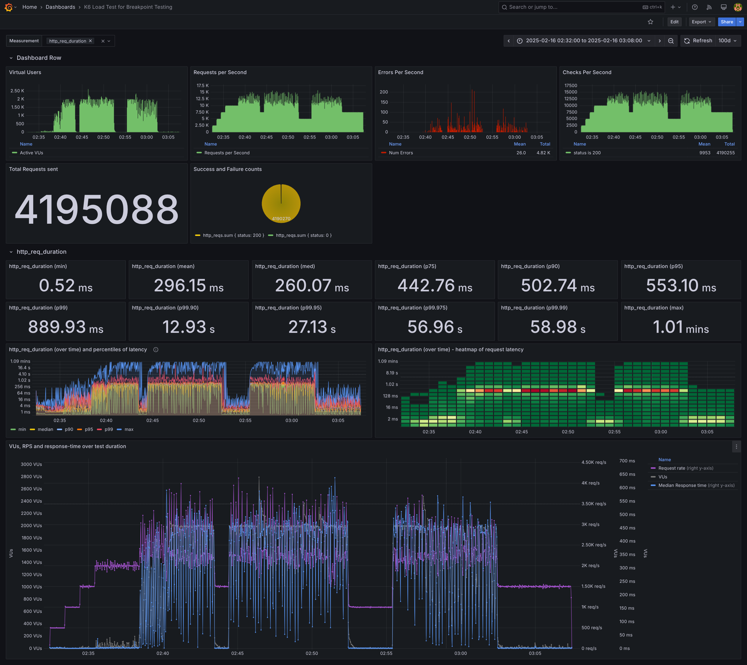
If everything is set up correctly, the Grafana dashboard should look like below and display http_req_duration by default. You can add other charts from the “Measurement” dropdown. Set the time range for queries at the top-right and increase the refresh interval (e.g., 100 days) to avoid unnecessary updates every minute you are going through the dashboard, as these can be slow when you have millions of requests. Note that numbers may slightly differ (by 1–2 decimal points) from K6’s stdout summary or K6’s HTML export due to SQL or grafana’s aggregations.

A quick tip: Some panels may fail to load. Instead of refreshing the entire dashboard, right-click a panel’s top-right corner → select View → click Refresh. If that doesn’t help, restart grafana-server.

Key Charts for Analysis

While I'll briefly mention all charts, I'll primarily refer to the following three for observations and conclusions:

1. Errors Per Second → Shows the number of failed requests (non-200 status) per second. Error spikes often align with RPS spikes.

2. http_req_duration (over time) and percentiles of latency → Displays min, median, p90, p95, p99, and max request durations every 4-second interval. This chart provides deep insights; feel free to add custom percentiles (e.g., p80, p99.95).

3. http_req_duration (over time) - heatmap of request latency → A heatmap of request latencies per minute. Unlike other panels, this does not use SQL queries but is computed entirely in Grafana, which can be resource-intensive.

   1. Color coding: Dark green represents a least number of requests (often only in few tens to few hundreds) → beige indicates a few more (a few dozen thousands) →with orange showing 70-80K and red showing the request volume above 90K.

   2. Helps determine how many requests complete within 512ms and how many exceed 1s, in a given 1 minute interval.

   3. On a c6a.4xlarge machine on AWS EC2, computing buckets for 21M requests didn’t complete even after 2 hours; on my laptop (with test of fewer VUs), ~4M requests took ~10 mins.

   4. If running long tests (several hours/days), x-axis granularity will change from 1 minute per unit.

Key Takeaways from Load Test Results

1. In the latency graph, until 2:38 (~6 min into the test), p99 remained below 128ms, as confirmed by both heatmaps and percentile charts.

2. In the heatmap, the first column on the x-axis shows that max latency was <128ms for only 43 out of 30K requests sent in the first minute (500*60). Of these, 29K+ requests completed in <8ms, with only 110 taking longer.

3. Continuing with the heatmap, hovering over the beige-colored areas up to 2:38 (~6 min in), only a few hundred requests exceeded 128ms. This corresponds to scenario-4 (multiplier 4, 500*4 RPS). Thus, this is the highest rate that avoids any errors. The failures chart shows that the first failure occurred at mid 2:38, when RPS increased by just 500.

4. From the heatmap, overall, ~97-98% of requests took <512ms, with only a few thousand exceeding that, reaching up to a minute or slightly more.

5. The highest failure spikes occurred at ~2:50, when base RPS hit 8x. This pattern repeated all three times we reached 8x, marking it as the degradation threshold—the point where failures surge.

6. From the heatmap, at 2:51, the heatmap shows a red square of 101K requests, most completing in <256ms. This pattern appears in all three instances of 7x base RPS, suggesting that 7x could be sustainable with an acceptable failure rate (a few hundred requests).

7. Interestingly, a couple of failures occurred during the cooldown period (2x for 3 min), while no failures were observed in the last 5 minutes (3x base RPS). This raises the question of whether earlier high loads had lingering effects—inconclusive.

Summary

• Stable points: Various RPS levels with zero failed requests and their corresponding latencies.

• Degradation point: The sharp rise in failures at 8x base RPS.

• Acceptable threshold: 7x base RPS with minor failures.

These insights should help determine whether to scale vertically or horizontally based on the latency and failure rates acceptable for your use case.

From static numbers and “VUs vs RPS vs median response time” graph:

1. From the Dashboard Row charts, the average request rate is 11K to 12.5K RPS, with mean and median latencies under 296ms—acceptable for my use case. Additionally, p99 latency across 4M+ requests is 890ms, which is great IMHO.

2. The max latency recorded is 1.02 seconds. To analyze what happened during that period, the "http_req_duration (over time) and percentiles of latency" chart provides insights. Several 59s spikes appear, but no 1.02 min instances. Since my test aggregates data every 4 seconds, the 1.02s latency instance may have been lost in aggregation. However, these 59s spikes occurred during peak load, likely due to the server queuing requests under high traffic.

3. The bottom chart, “VUs, RPS, and median response time” confirms an earlier point, avoiding 20x-50x spikes and sticking to 8x base RPS. As seen here, VUs maxed out at just 3x base RPS, reinforcing the need for careful scaling of VUs and being midful of the resources on which the load test is being run.

Extrapolating these learnings

1. DNS & TLS Overhead: Ensure that K6’s built-in DNS caching is not masking real-world lookup times. Set the flg --dns to 0 to disable DNS cache and read about that flag in k6 run --help to learn more.

2. Client-side Bottlenecks: If the K6 test machine lacks enough network bandwidth, CPU, or memory, it may become a bottleneck rather than the backend server being tested. Monitor K6’s internal metrics, vus, http_req_blocked, http_req_failed, etc. to figure out this part. The chart in the bottom for other ‘measurements’ could help here.

3. Backend Auto-scaling: If the backend auto-scales, ensure the results reflect a steady-state rather than transient behavior due to infrastructure scaling.

4. Queueing Effects: If response time degrades significantly (e.g., >1 minute), check if requests are queuing internally due to exhausted resources (e.g., database connections, thread pools).

5. Cold Start Effects: Run a warm-up phase before starting actual tests, especially for cloud services, to avoid cold start latencies skewing results.

6. Network Variability: Run tests multiple times to identify variance due to network jitter or congestion.